With the widespread conversion of the TV transmission and coding standards, from the early analog (NTSC, PAL, SECAM) systems to the modern digital formats (ATSC, DVB, ISDB, etc.), added to the price reduction of larger screen devices, old analog TV sets have become obsolete, unless they are used with converter boxes or connected to analog content generators, such as video game consoles with analog output. Here I will present a method to generate NTSC TV synchronism signals, so the old analog TV sets can be used again to show user-generated content.
Analog television operation is regulated by norms and standards, which assure compatibility between the signal generation, transmission, reception and finally reproduction on a TV screen (see “Video Pattern Generator” on the Projects section for a complete description of the theory behind the TV transmission and the practical solutions that ended up in the main analog standards being created).
For an image to appear complete and perfectly stable on a TV screen, it must comply with very strict timing requirements, which vary among the various standards. These timing requirements are usually known as “synchronism pulses”, and are divided into two main components: Vertical and Horizontal.
The vertical synchronism indicates when a new image field starts; the horizontal, when each one of the lines composing the field starts. Both synchronisms can be sent separately or joined together, known as “composite synchronism”, which is the usual way in which a TV set receives this signal.
The composite synchronism can be generated with any clocked circuit that can count clock pulses; therefore it seems a task fit for a microcontroller. Let’s see how to generate a complete NTSC-M composite synchronism using a PIC microcontroller (PIC 12F1571), programmed in C language using the CCS C compiler.
NTSC-M composite synchronism
The NTSC-M standard image is composed of 525 horizontal lines, shown as two consecutive fields of 262.5 lines each. The start of each field is marked by the vertical synchronism, preceded by the pre-equalizing pulses and followed by the post-equalizing ones.
The duration of the pre and post-equalizing pulses, as well as the vertical synchronism, is equal to 3 horizontal lines each block; therefore, 9 horizontal lines are always used to generate these pulses. The spacing between each pre and post-equalizing pulse is half of a horizontal line, so 6 pulses are generated in each group. The vertical synchronism includes the serrated pulses, also spaced half horizontal line (Figure 1).
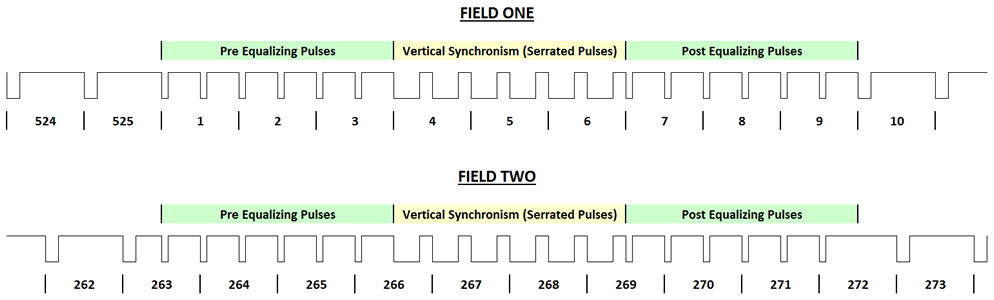
FIGURE 1. – Start of fields one and two; the line numbers are written below each line
As mentioned before, each field has 262.5 lines, so the last line of the first field is just one half of a horizontal line, as well as the first line of the second field. This fact guarantees that the lines appear on an interlaced fashion on the screen, creating the so called “interlaced scanning” (Figure 2).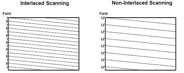
FIGURE 2. – Interlaced and non-interlaced scanning
The other method to scan the image is the “non-interlaced scanning”, also called “progressive scanning”. Normal TV transmission uses the first method, while the progressive scanning is used when showing static patterns, such as text or graphics, since the interlaced method will produce vertical jitter.
After the post-equalization pulses, the standard horizontal lines are generated. It is possible to insert video in each of these horizontal lines; however the standard indicates that there should be a “vertical blanking period”, which goes up to line number 20. During this period there is no video inserted, just pure synchronism. This is fine, since these lines will fall outside the visible screen in any well-adjusted TV set.
After line 20, the video information can be added to the synchronism pulses. There are however some timing considerations, as shown in Figure 3.
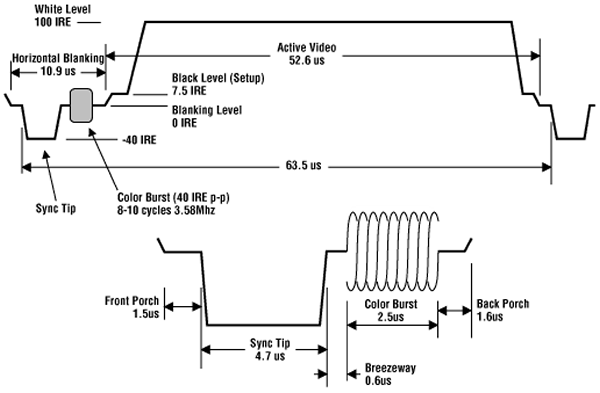
FIGURE 3. – Horizontal line, showing the detailed timing of the horizontal synchronism and surrounding elements
The horizontal pulse duration is 4.7 µs (shown as “Sync Tip”), preceded by the “Front Porch” (1.5 µs) and followed by the “Back Porch” (4.7 µs). This back porch will contain the color burst in case of a color transmission, so it is shown as “Breezeway”, “Color Burst” and “Back Porch”; for a black and white image, this breakdown is not relevant. After this, the video information will be sent, and it may last until the next front porch arrives. Since the horizontal frequency is 15,734 Hz, the total line duration is close to 63.55 µs; subtracting the time used by the synchronism pulse and both porches, the useful video window is around 52.65 µs, which fits in the visible screen.
Generating the composite synchronism in C
As previously seen, the synchronism generation is a matter of timing; count the appropriate number of clock pulses and set a microcontroller pin up or down, as required. Repeat this as many times as there are lines in a frame, and you have a complete composite synchronism.
While in assembler we may have a complete control of the timing, since we are counting machine instructions, in C the scenario is completely different. The number of machine instructions generated by a given C command will depend largely on the compiler used and the optimization level it may reach. However, there is a very precise way to generate a timing reference: using the PIC timer interruption.
Before start analyzing the program, let’s take a look at the hardware, shown in Figure 4.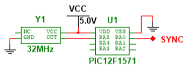
FIGURE 4. – Synchronism generator schematic
The setup is extremely simple: a clock generator and a PIC. You may notice, by reading the datasheet, that this PIC can generate the clock internally, so there is no need for the external oscillator. While this is true, the internal oscillator is not stable enough to produce accurate timings, and there will be a noticeable wobbling in the generated image. Therefore, an external crystal oscillator is required.
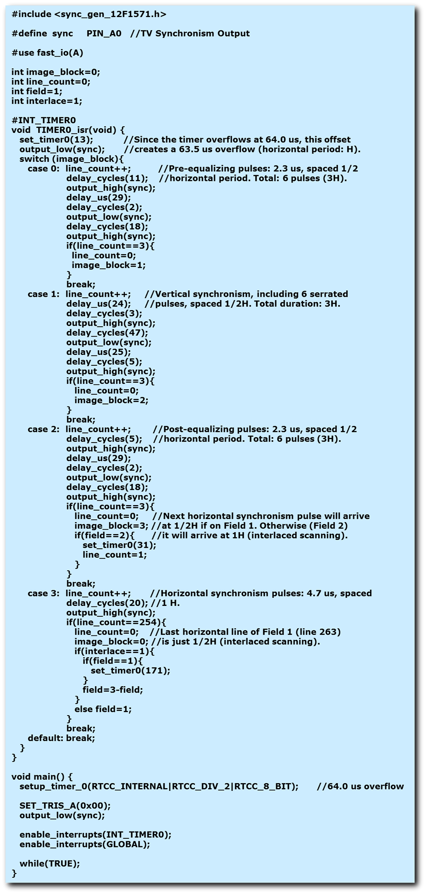
The system clock frequency is set at 32 MHz; this frequency is perfect for our purposes. Setting the Timer0 (8 bit timer) to be updated every 2 instruction clock pulses (32 MHz / 4 = 8 MHz), it will overflow exactly at 64 µs [(1 / 8 MHz) x 2 x 256]. Therefore, the Timer0 interruption will be triggered every 64 µs.
This is the program configuration:
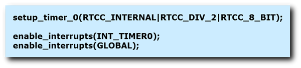
While 64 µs is quite close to the horizontal period, we can increase the precision to achieve 63.5 µs; it only requires loading the Timer0 with an offset value, so it reaches the overflow value in less than 64 µs. This is the first thing to do when the interruption is called:
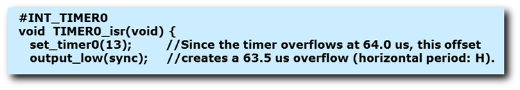
The Timer0 is loaded with 13. If we calculate the new interruption timing, the equation is as follows: (256-13) x 0.25 µs = 60.75 µs. This is much less than the required 63.5 µs; however, when we put together the time required for the program to service the interruption, save context variables and execute this initial instruction, the result is 63.5 µs. This is one of the drawbacks of programming in C as mentioned before: you do not know what the compiler is actually doing. So this value is adjusted by carefully observing the generated signal in an oscilloscope. This is not even constant from one PIC family to another; if using the PIC16F1825, this value should be 15 instead of 13.
In any case, we have just set the most important time reference: the horizontal period. Every 63.5 µs the interruption will be called and the horizontal synchronism pulse will be initiated [output_low(sync);].
Earlier in the program I defined the Pin A0 (RA0 in the schematic diagram) as the synchronism output, so I can now refer to it simply as “sync”.
It is standard practice not to remain inside an interruption routine for a long time, so the program can continue with the other tasks. In our case, the main task assigned to the PIC is to generate the synchronisms, so we will remain inside the interruption as much as needed to guarantee a controlled and precise timing.
Now it is time to generate the different pulses, starting with the pre-equalizing block. A variable called “image_block” will control in which block we are, while another called “line_count” will count the lines generated inside each block.
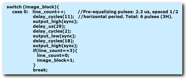
Each pulse lasts for 2.3 µs, and are spaced half a horizontal line. Delaying 11 instruction cycles before moving up the sync pin again produces the 2.3 µs pulse, and the spacing is achieved by delaying 29 µs and 2 cycles. Another pulse is generated; now 18 cycles are required to achieve the 2.3 µs since there are no other instructions in the middle. After that, leave the interruption routine and return when it is time for a new horizontal period start.
The process continues until line_count reaches 3; at this point (end of pre-equalizing block) the line_count is reset and the image_block is increased by 1, indicating the start of the next block.
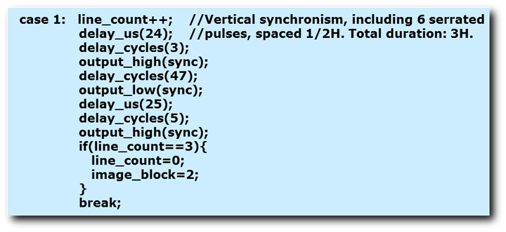
The vertical synchronism block follows the same logic; the main difference is that now the sync pin stays low during a longer period, and only returns to the high state to generate the serrated pulses. After 3 lines, line_count is reset and image_block is loaded with 2.
Now it is time to generate the post-equalizing pulses; same logic as before, with one fundamental change: the field detection to implement the interlaced scanning.
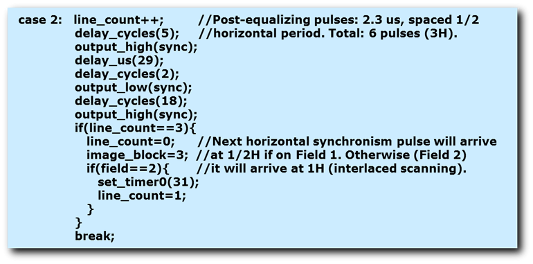
The first 3 loops are almost identical to the generation of the pre-equalizing pulses; only the duration of the first pulse in each loop has been reduced to 5 cycles (instead of 11), to compensate for the delay to reach this block (in a “switch” statement, each successive “case” represents a 3 cycle delay). With this precaution, the actual pulse maintains the 2.3 µs duration.
When line_count reaches 3, then the variable is reset, the image_block loaded with 3 and a new variable is evaluated: “field”. If field is 1, then the next horizontal pulse will arrive at half the horizontal period, when the interruption is triggered (line 9 in Figure 1). So, there is nothing to do here. However, if we are in the second field, in order to maintain the half-line shift on the interlaced scanning, the next horizontal pulse needs to arrive one complete horizontal period after the last post-equalizing pulse (line 272 in Figure 1). Therefore, the Timer0 is loaded with a new value in order to achieve this longer period, and line_count loaded with 1 instead of 0, to maintain the total count (field 1 + field 2) equal to 525 lines.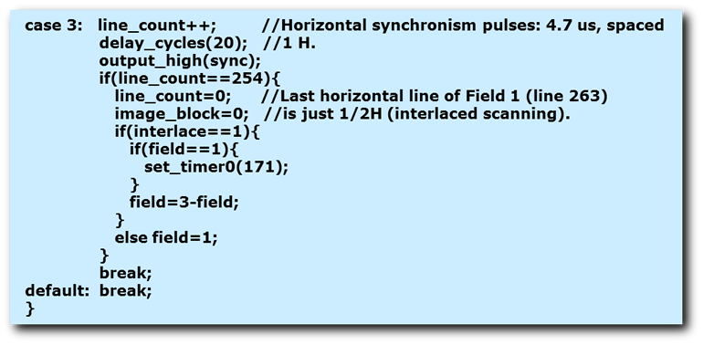
The last block (case 3) generates all the rest of the horizontal lines; this is the “blank canvas” where the video content will be added to be shown on the TV screen. Using a 20-cycle delay the 4.7 µs horizontal pulse is generated, and the program leaves the interruption routine. This is until line 254 is reached (lines 263 or 525 in Figure 1). At this point, line_count and image_block are both reset, and a new variable is evaluated: “interlace”. If interlace is 1 (meaning “interlaced scanning”), then “field” is evaluated; if in field 1 (line 263 in Figure 1), the next pre-equalizing pulse will arrive only one half horizontal period later, so Timer0 is loaded accordingly (171). If in field 2 (line 525 in Figure 1), Timer0 remains untouched (one complete horizontal period will be generated). In both cases, the variable “field” is toggled to keep the interlace process running.
If interlace is 0, however, field is always loaded with 1. In this case, the field 2 is never generated, and field 1 repeats itself every time. This will create the “progressive” or “non-interlaced scanning”.
At this point, the full program has been described. When powered, the “sync” pin (RA0) will output a perfectly timed composite synchronism, to be used in any TV with the NTSC-M system. Here is the full program, written using CCS C:
 (
(The configuration file (sync_gen_12F1571.h) includes the external oscillator definition:
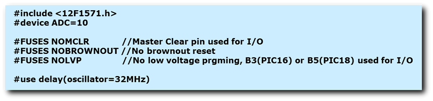 (
(Figure 5 shows an actual capture of the signal being generated. The trigger is locked at line 1, so the pre and post-equalizing pulses can be seen, as well as the vertical synchronism between them, and the last and first horizontal lines on both extremes of the oscilloscope screen. This is the end of field 2 (line 525) and the start of field 1 (line 1). The first horizontal synchronism of field 1 (on the right) arrives half line after the last post-equalization pulse.

FIGURE 5. – Signal locked at line 1, showing the transition from field 2 to field 1
Figure 6 shows the end of field 1 and the start of field 2. The trigger is locked at line 263; this is just a half line, followed by a pre-equalizing pulse. In order to maintain the total line count equal to 525, the first horizontal synchronism arrives at one full line after the last post-equalization pulse, as can be seen on the right side of the image. This is typical of an interlaced scanning, as previously explained.
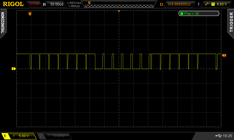
FIGURE 6. – Signal locked at line 263, showing the transition from field 1 to field 2
While the timing is perfect, this signal is not suitable yet to be connected to a TV receiver through the video input. You may notice that the amplitude is 5.0 V, and the video input standard requires 1.0 Vp-p (including the video content, not shown here), so further amplitude shaping will be required.
The main purpose of this generator is to feed another circuit (e.g. another microcontroller) with the proper synchronisms, so this second circuit does not have to worry about timing, just generate the proper video contents and insert them within the video window (52.6 µs, as previously seen). This signal can also be used as the reference to scan a video memory, so its contents are sent sequentially to the TV, to form a complete image. This is the principle behind the “TV Character Generator” presented on the Shop section.
Practical examples
While this program’s primary use is to just generate composite synchronism, it can be used as a standalone TV generator, if proper care is taken not to interfere with the timing. Let’s start by adding some components to the circuit schematic, as shown in Figure 7.
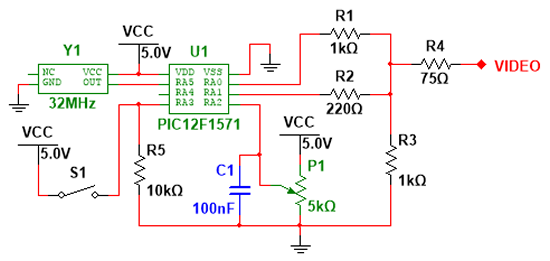
FIGURE 7. – Modified circuit schematic
This new circuit has a few added improvements:
- Besides synchronism (RA0), it will generate a video component in RA1.
- Four resistors (R1 through R4) add the synchronism and video signals, and adjust the amplitude to the TV video input requirements.
- A variable resistor (P1) connected to an analog input (RA2) will let us modify the video component.
- The switch (S1) connected to RA3 will let us select the scanning method.
In order for these changes to work, the program requires some additions. First of all, we will add a pin definition and a new variable:

Then, the main program needs to be modified:
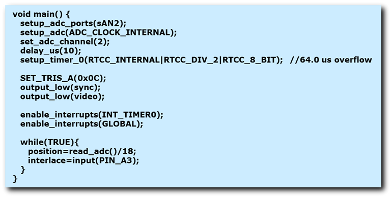
Basically, the ADC configuration is done for RA2 (sAN2), the proper direction of the Port A pins is set and all the outputs cleared. Within the main loop, the new variable “position” will receive the value of the ADC divided by 18 (maximum would be 1024 / 18 = 56), and “interlace” will be equal to the state of RA3 (PIN_A3). Therefore, the switch S1 will control the scanning method directly, ON = interlaced, OFF = progressive.
Finally, the horizontal lines block (case 3) will include the video generation:
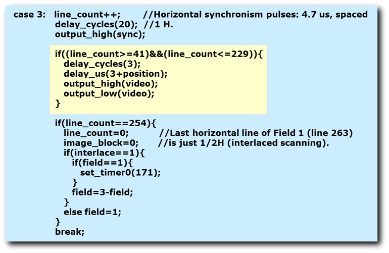
The highlighted section generates the video signal: from line_count = 41 to line_count = 229, a vertical line will appear on the TV screen. The horizontal position of this line will be controlled with the variable resistor (P1), moving 1 µs at a time. The offset (3 cycles + 3 µs) prevents the line to step over the back porch.
In brief, to show anything on the TV screen, the vertical position is obtained by selecting the appropriate horizontal lines, while the horizontal position is determined by the time delay from the synchronism pulse.
If we would like to draw a wider vertical line, we only need to add some delay between the “output_high(video);” and the “output_low(video);” instructions. An extreme case would be to put the position in 0 and increase the line width to cover the whole video window: the result would be a white screen, at least within the horizontal lines selected to insert video.
Figure 8 shows the actual TV image with the line positioned around the center of the screen; Figure 9 shows the oscilloscope trace triggered at scan line 50 (line_count = 41).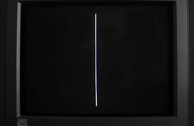
FIGURE 8. – Vertical line at center of TV screen
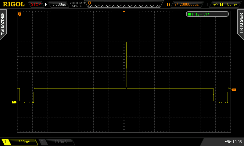
FIGURE 9. – The uppermost dot of the vertical line as seen on the oscilloscope
Turning P1 clockwise, the line can be moved to the right, as shown in Figures 10 and 11.
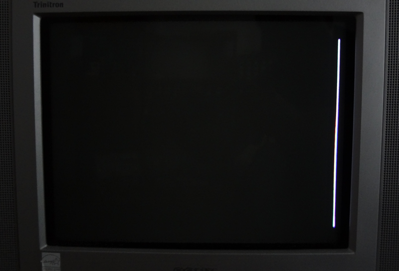
FIGURE 10. – Vertical line moved to the right
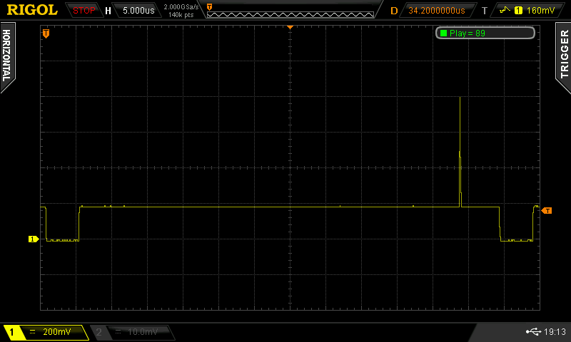
FIGURE 11. – The line position on the oscilloscope
How far to the right can we go? Besides the standard definition, which indicates that there must be a separation of 1.5 µs from the next horizontal pulse (Front Porch), there is a practical limitation related to the way we are generating these pulses. Since we are inside an interruption service routine, with the interruption disabled, we need to make sure that the program leaves the routine before the next interruption comes. This is not an instantaneous task, so a few microseconds must be considered to be on the safe side. As a matter of fact, the line in Figures 10 and 11 is located at the rightmost position that guarantees a correct timing. This position is about 5.5 µs from the next horizontal pulse; considering that the Front Porch takes 1.5 µs, then we are effectively losing 4.0 µs of the video window.
In practical terms this is not an issue; a good part of these 4.0 µs is effectively not visible in most TV sets, and we must always guarantee a safe zone to show text and graphics. Therefore, there is no practical reason to even try to show anything in this zone.
In any case, what happens if we try to move further to the right? Figure 12 shows the answer.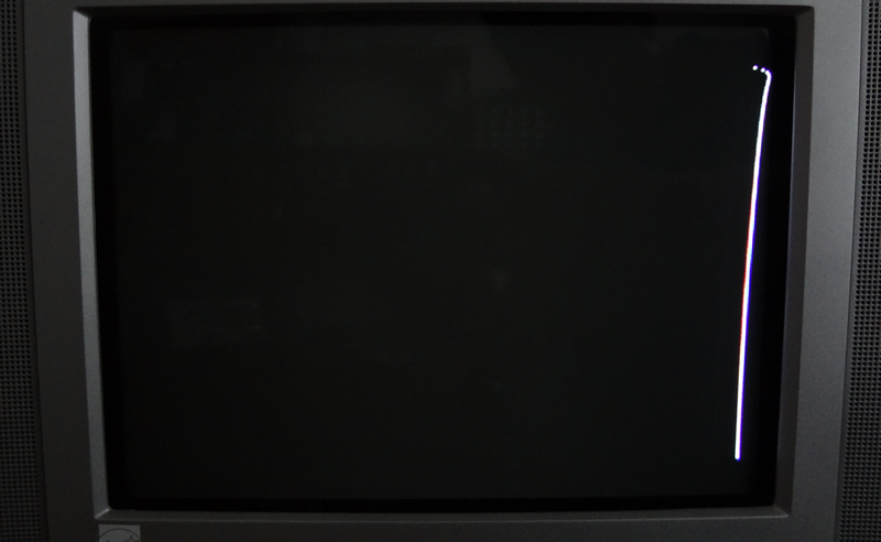
FIGURE 12. – Distorted timing due to delayed interrupt servicing
Since the interruption cannot be serviced at the precise time, the horizontal line gets longer, distorting the top of the vertical line. With successive horizontal lines the TV circuits eventually lock into the new timing, but the distortion reappears at the end of the line, not visible here since the screen is black and there is no other pattern.
Obviously this limitation will not happen if this PIC is just dedicated to generate the synchronisms and there is another circuit dedicated to generate the video; however it is good to know how it works.
How far to the left can we go? There is no limitation here in terms of the program, we just need to make sure that the Back Porch is not overwritten with video, and that we are within the safe text and graphics zone. Figures 13 and 14 show the line on the left edge of the screen: almost entering the invisible zone.
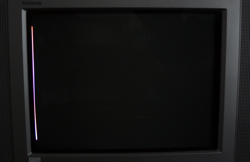
FIGURE 13. – Vertical line at the leftmost visible position
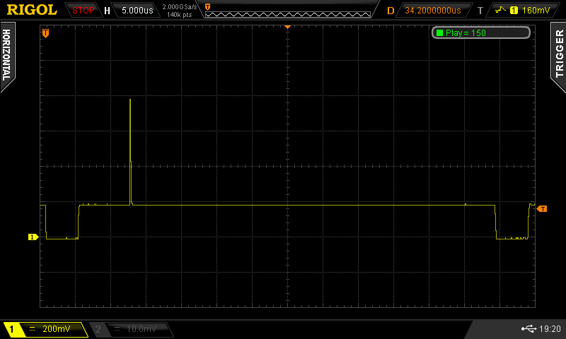
FIGURE 14. – The same line as seen on the oscilloscope
This experiment lets us draw some interesting conclusions about the synchronism generation and the visible screen area.
In Figure 3 we learned that the video content may start right after the Back Porch, about 4.7 µs from the end of the horizontal synchronism pulse. Looking at Figure 14, it is evident that the image starts to be visible on screen around 7.5 µs after the pulse. This will vary depending on the actual TV adjustments, and some units may show a bit more, others a bit less. So it is very important to consider the safe zone I mentioned before when planning to show text and graphics. For standard TV transmission, of moving images, this fact may not be very relevant, since the action is mostly centered on the screen, with not much important content on the sides.
To finish, let’s draw a rectangle on the screen, to show graphically a reasonable safe zone.
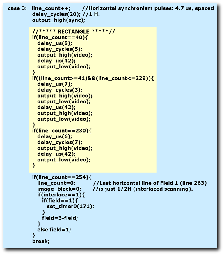
Using the same principles previously shown, we draw a horizontal line, then two vertical lines, and finally a new horizontal line: this is a rectangle. Figure 15 shows this new image.
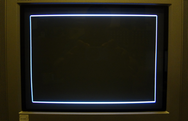
FIGURE 15. – Rectangle on screen, showing the limits of a reasonable safe zone to insert text and graphics
The top and bottom lines can be seen like Figure 16 on the oscilloscope; they are located at scan lines 49 and 239 on field 1, and the corresponding lines on field 2 (if interlaced).
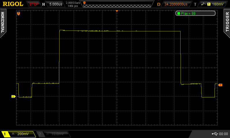
FIGURE 16. – Top and bottom lines of the rectangle
The vertical lines show a familiar pattern, but now with 2 lines instead of 1, as seen on Figure 17.
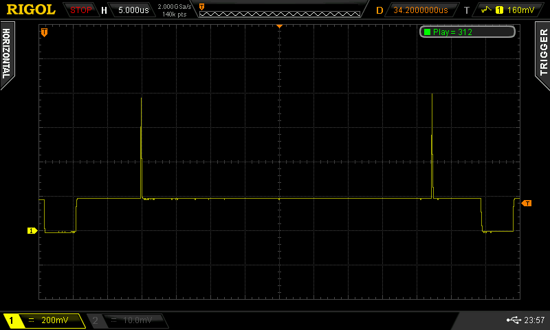
FIGURE 17. – Side vertical lines of the rectangle
In conclusion, a reasonable safe zone for displaying text, charts and graphics, should be around these numbers:
- Upper limit: scanning lines 44 to 49 on field 1, and the equivalent on field 2 (lines 306 to 311).
- Lower limit: scanning lines 239 to 244 on field 1, and the equivalent on field 2 (lines 501 to 506).
- Left limit: 9 to 10 µs from the end of the horizontal synchronism pulse.
- Right limit: 6 to 7 µs from the beginning of the next horizontal synchronism pulse.
With these limits in mind, the maximum usable screen size would be 200 horizontal lines in the vertical dimension, and around 44 µs horizontally, which gives a reasonable area to show information. Just for reference, the “TV Character Generator” mentioned before uses a grid of 320 pixels horizontally, by 192 vertically. Since each pixel lasts 1 instruction clock (0.125 µs), the horizontal time is 40 µs. In the vertical dimension, each pixel is a horizontal line, so there are 192 lines used. The resulting screen is well within the defined safe zone.
One last comment regarding the use of interlaced or progressive video; as mentioned earlier, the progressive scanning is preferred when showing text and graphics, since the interlaced method produces vertical jitter. This happens because the equivalent lines in field 1 and 2 appear in slightly different positions when composing a complete frame and the eye perceives this movement when showing static images. The progressive method does not have this problem, since there is only one field that repeats over itself continuously; the drawback is the reduction in vertical resolution to one half of the interlaced scanning. This generator offers both options, for added flexibility.