Distance can be measured in various ways: directly, using a ruler or measuring tape, or indirectly, using radio or sound waves. The indirect method measures another variable (e.g. time), in order to calculate the distance. Here we will review a practical way to measure short distances (2 cm up to 4 m) using ultrasonic waves.
Sound waves travel through different materials by compressing and expanding the molecular arrangements (Figure 1).

FIGURE 1.- Sound waves traveling from a source (speaker) to a receiver (microphone)
Therefore, sound waves:
- Can only travel through a physical medium (no sound in vacuum).
- Will travel at a speed that varies with the material, based on the various molecular structures.
We will be using sound waves traveling through the air, so all the calculations will be based on this fact.
These waves can be characterized by 2 parameters: amplitude and frequency. Sound waves, in the most common definition, have a frequency range varying from 20 Hz to 20 kHz, which is the human audible range. However, it is possible to generate waves below or above this frequency range; the latter are called “ultrasonic” waves.
The use of ultrasonic waves is quite practical since they show the same behavior of any sound wave but do not annoy the user since they are outside the audible range. Be careful, however, since your pets (particularly dogs) may be quite sensitive to these waves.
Time as a measure of distance
There is a fundamental equation that relates Speed, Distance and Time:
SPEED = DISTANCE / TIME
So the speed at which any object is moving is directly proportional to the distance traveled and inversely proportional to the time consumed to reach the destination. In brief, an object moves faster as it covers more distance in less time.
The same equation applies to sound waves; in this sense, knowing 2 of the variables would be enough to calculate the third.
The speed of sound in the different materials can be calculated knowing the various properties of the material; in case of dry air, the speed in meters per second (m/s) can be obtained using the following equation:
SPEED = 331.4 + 0.6 x Tc
Tc is the temperature measured in Celsius. This equation is quite precise for temperatures close to the ambient temperature (25 °C), and a more complete formula should be used for much lower or higher temperatures (e.g. 200 °C). For our purposes, we will consider a living environment range (10 °C to 40 °C), so the previous equation will be used.
So, we have the speed, how do we obtain the time? This is quite simple. In Figure 1, we just need to start the clock when the sound leaves the speaker, and stop when it arrives to the microphone. This setup, however, requires that we have synchronized circuits at both ends of the distance to measure, which is not very practical; Figure 2 shows a more usable setup.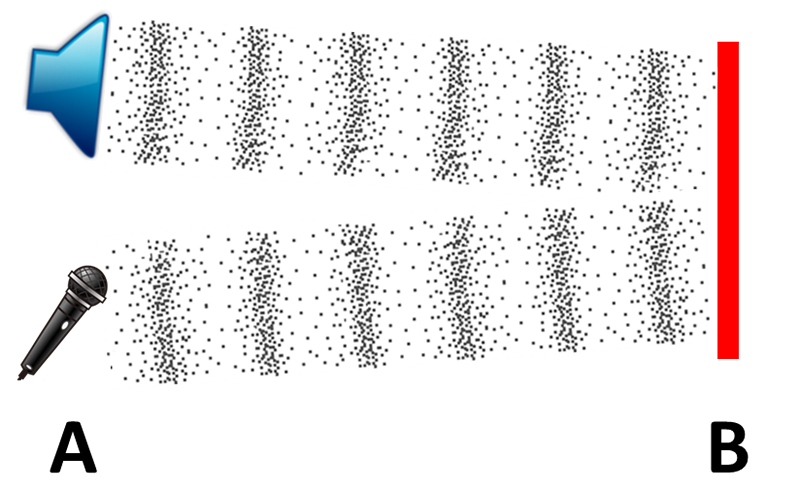
FIGURE 2.- The microphone captures the sound waves reflected by the object located at B
With the sound source and receiver on the same side, it is much easier to control and monitor both with a single circuit, simplifying the time measurement task.
Now, with the speed and time known, the distance between A and B can be calculated as:
DISTANCE = SPEED x TIME / 2
We need to divide by 2 the result since we are measuring the time from A to B and back to A, which is twice the distance we are trying to determine.
Therefore, we have demonstrated that the distance between 2 points can be calculated by measuring the time it takes for a sound wave to travel between them.
Practical implementation
At this point we may start gathering a speaker, a microphone, some amplifiers and control circuits to simulate the scenario shown in Figure 2. Fortunately, there is no need to do this, since there are inexpensive solutions already available that we may use to simplify the task.
Figure 3 shows an ultrasonic distance sensor module that incorporates the speaker, the microphone and the required electronics to measure the sound travel time.
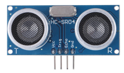
FIGURE 3.- Ultrasonic distance sensor module, HC-SR04
This device has 4 terminals; there are other modules with 3 terminals, with similar performance. However, the price of the 4-terminal units is only a fraction of the others; therefore I will be using these modules. If you prefer to use a 3-terminal module, the concepts are the same and just minor changes should be made in the setup and program.
Besides Vcc and GND (these devices work on 5.0 V), there are 2 other terminals named “Trig” and “Echo”. The names are quite indicative of their function: “Trig” (trigger) receives a pulse to initiate the generation of the sound wave, while “Echo” outputs a pulse equal to the duration of the wave travel.
Figure 4 shows the timing requirements and the working principles of the module.
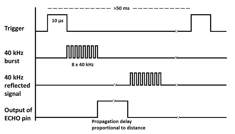
FIGURE 4.- HC-SR04 timing requirements
The operation is initiated by sending a 10 µs pulse to the Trigger terminal. The module internally generates a burst of 8 cycles at 40 kHz (ultrasonic) sent by one transducer (T - speaker). The Echo pin goes high until the burst is received back on the other transducer (R - microphone). The operation can be repeated indefinitely, provided there is a separation of at least 50 ms between triggers.
The process control and signal processing can be achieved with a microcontroller, as shown in Figure 5.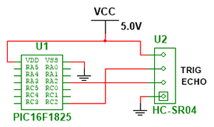
FIGURE 5.- A PIC 16F1825 can be used to control the HC-SR04
Using a PIC 16F1825, configured with the internal clock, there is no need to add any other component to perform the module test. The communication is achieved with 2 pins, RC2 connected to the Trigger and RA2 receiving the signal from Echo. The selection of RA2 is not random; this pin is the External Interrupt Input of this PIC, and we will be using it in our program.
Basic program
In order to control the ultrasonic module and measure the resulting propagation delay, the program must:
- Send a pulse (10 µs or longer) through RC2.
- When RA2 becomes HIGH (Echo initiated the pulse) start a counter.
- When RA2 becomes LOW (Echo terminated the pulse) read the counter contents.
- Restart the process after 50 ms or more.
This basic routine will give the total travel time of the sound wave (going and returning back). Knowing the speed of sound, as discussed above, it is just a matter of a simple calculation to determine the distance to the object where the wave bounced.
Here is the program in CCS C: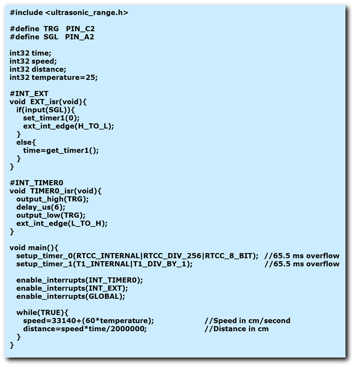 (
(And this is the configuration file (ultrasonic_range.h):
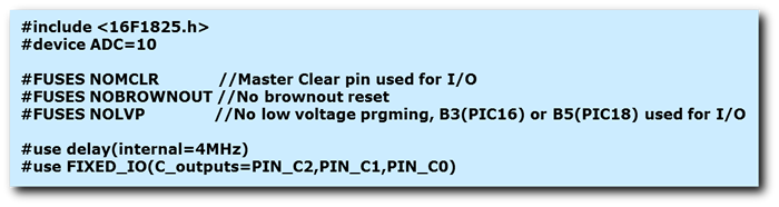 (
(The first thing to notice is that the PIC is using the internal oscillator at a relatively low speed (4 MHz); this is on purpose, to achieve very long time periods with the Timer0 and Timer1.
In the main program, Timer0 (8 bits) is set to increase 1 count every 256 instruction clock pulses. Given that the instruction clock period is 1 µs (4 times the oscillator period) then Timer0 is increased every 256 µs. Therefore, Timer0 will overflow at 256 increments x 256 µs/increment = 65536 µs (approximately 65.5 ms as noted in the program comments).
Timer1 (16 bits) is increased with every instruction clock pulse, so it will overflow at 65536 increments x 1 µs/increment = 65536 µs. With this configuration, both timers overflow with the same interval.
Two interrupts are enabled: Timer0 and External. Timer0 interrupt is triggered every time the timer overflows, therefore the ISR (Interrupt Service Routine) will be called every 65.5 ms. We will use this ISR to trigger the ultrasound module; as you may recall, there should be at least 50 ms separation between cycles, so 65.5 ms is perfect for our purposes. Inside the Timer0 ISR the TRG pin (RC2) is raised, wait 6 µs and then lowered. You may wonder why only 6 µs if the trigger pulse must be 10 µs or more? The other instructions take time as well, so the actual pulse duration is in fact 10 µs.
After this, the External Interrupt Edge is set, waiting for a LOW to HIGH transition from the Echo pin on RA2. The program leaves the ISR and continues inside the while(TRUE) loop.
When Echo starts the measuring pulse, so a LOW to HIGH transition appears in RA2, the External Interrupt ISR is called. Since RA2 is now HIGH, then Timer1 is reset (starts in 0), and the Interrupt Edge is now set from HIGH to LOW. The program leaves the ISR.
The sound wave will eventually reach the module after bouncing with the object, so Echo will go LOW. This transition triggers the External Interrupt again, but now RA2 will be LOW. At this point, the variable time will receive the contents of Timer1: this is the total travel time in µs.
If the sound wave never returns, i.e. there is no object to bounce, the Echo pin will return to LOW after 38 ms, so the program will always update the variable time, but we must be aware that any time longer than 25 ms should not be considered as a valid measure.
To understand this previous statement, let’s review the next steps in the program. Within the while(TRUE) loop, speed is calculated using the equation previously presented:
SPEED = 331.4 + 0.6 x Tc
The only difference is that instead of meters per second (m/s) we are using centimeters per second (cm/s), so both terms of the addition are multiplied by 100. This has an obvious advantage: we keep precision without using floating point numbers, so everything is faster and uses less memory. The variables must be defined as int32.
The temperature has been set as 25 °C, and may be changed if desired. The ideal setup should include a temperature sensor connected to the PIC, so the actual ambient temperature is used.
The distance can now be calculated by multiplying speed and time, divided by 2 (to measure only one way of the sound trip). Six zeros are added to convert the time from µs to s. The result is given in centimeters (cm).
Back to the previous statement, that any time longer than 25 ms (or 25,000 µs) should not be considered a valid measure, let’s calculate the distance for this time (at 25 °C):
Distance = (33,140 + (60 x 25)) x 25,000 / 2,000,000 = 433 cm
The HC-SR04 datasheet indicates a maximum range of around 4 m (400 cm), so 433 cm may be possible, but the results are not guaranteed beyond that point.
What’s next?
With the distance already calculated and stored in the variable distance, the next step would be to do something with the information. This is limited only by the imagination (or actual needs) of the user, and it can go from showing the results in an LCD alphanumeric or graphic display, to transmitting the results via radio signals to a remote location or even showing them in a web page. The sensor could be mounted in a servo mechanism that oscillates covering half a circle, thus creating a sonar device.
The applications are endless, using this low cost module and the simple program described above.